土壤

Table of contents

背景
CCTM 所需土壤數據
Reading the isric tiff’s (CEC and PH)
Reading 2015 250m resolution Global GeoTiff’s
Porosity
Reference

背景

soilgrids是位於荷蘭世界土壤資訊機構isric.org轄下SoilGrids及WoSIS專案成果展示之互動地圖，該網站亦提供了全球土壤GIS資料庫，最高解析度達到250M，時間範圍自1997至2020。
- 以方磚方式儲存，如
- 項目有：bdod, cec, cfvo, clay, landmask, nitrogen, ocd, ocs, phh2o, sand, silt, soc(Soil Organic Carbon), wrb
- 30秒數據
- 2015年全球GeoTiff
Our World in Data全球長期的土地使用、農業、肥料與作物土地面積等數據。解析度為國家。
Ramankutty, N., Evan, A.T., Monfreda, C., and Foley, J.A. (2008). Farming the planet: 1. Geographic distribution of global agricultural lands in the year 2000. Global Biogeochemical Cycles 22 (1). doi:10.1029/2007GB002952.
- Data distributed by the Socioeconomic Data and Applications Center, NASA (SEDAC)
- 數據為2000年基準，單位為農地面積比例，解析度為5分~10Km。資料格式為geoTiff、ESRI gridfile。
- Data presented as five-arc-minute, 4320 x 2160 cell grid, Spatial Reference: GCS_WGS_1984, Datum: D_WGS_1984, Cell size: 0.083333 degrees, Layer extent: Top : 90, Left: -180, Right: 180, Bottom: -90 earthstat.org
- Harvested Area and Yield for 175 Crops, earthstat.org

CCTM 所需土壤數據

控制選項

E2C_SOIL – EPIC soil properties
- Used by: CCTM – bidirectional NH3 flux version only
E2C_CHEM – DAILY EPIC crop types and fertilizer application
- Used by: CCTM – bidirectional NH3 flux version only

檔案結構

layer有42個，為各作物種類數(e2c_cats)。
- 因網格內同時有多種作物，因此土壤有種植該作物時對應之性質。
- 會對應到土地使用檔中的穀物面積分率

$ nc=/home/cmaqruns/2018base/data/land/1804/2018_EAsia_81K_soil_bench1804.nc
$ ncdump -h $nc|H
netcdf 2018_EAsia_81K_soil_bench1804 {
dimensions:
        COL = 53 ;
        TSTEP = 1 ;
        LAY = 42 ;
        ROW = 53 ;
        VAR = 13 ;
        DATE-TIME = 2 ;

變數名稱及內容

層數：L1(0 to 1 cm depth) and L2 (1 cm to 100 cm depth)
‘SoilNum’：放在L1之下：’L1_SoilNum’
各層變數含SoilNum共7類：

var. name	desc	unit	range	usage	link
SoilNum	Soil Number	-	1~8005	(not found)
Bulk_D	Bulk Density	t/m**3	0.85~1.67		bdod
Cation	Cation Ex	cmol/kg	1.03~48.82	cec1~2(ncols, nrows, e2c_cats) in depv_data_module	cec
Field_C	Field Capacity, Water holding capacity, water retention capacity	m/m	0.07~0.48	(not found)	LSM_MOD.F:!– WFC is soil field capacity (Rawls et al 1982)available water capacity (-33 to -1500 kPa)
PH	potential of H ions	-	5.36~ 7.47	pHs1~2	phh2o
Porosity	Porosity	%	0.2~0.55	por1,por2 in module depv_data_module		total porosity
Wilt_P	Wilting Point	m/m	0.03~0.32	wp1~2	soil water capacity (volumetric fraction) until wilting point

number of soil type in LSM_MOD.F

      INTEGER, PARAMETER :: N_SOIL_TYPE_WRFV4P = 16
      INTEGER, PARAMETER :: N_SOIL_TYPE_WRFV3  = 11

METCRO2D_1804_run5.nc SLTYP:var_desc = “soil texture type by USDA category “

e2c categories number in depv_data_module.F

! depv_data_module.F:32:
            integer, parameter :: e2c_cats = 42   ! number of crop catigories

lookup tab of LSM_MOD.F

C-------------------------------------------------------------------------------
C Soil Characteristics by Type for WRF4+
C
C   #  SOIL TYPE  WSAT  WFC  WWLT  BSLP  CGSAT   JP   AS   C2R  C1SAT  WRES
C   _  _________  ____  ___  ____  ____  _____   ___  ___  ___  _____  ____
C   1  SAND       .395 .135  .068  4.05  3.222    4  .387  3.9  .082   .020
C   2  LOAMY SAND .410 .150  .075  4.38  3.057    4  .404  3.7  .098   .035
C   3  SANDY LOAM .435 .195  .114  4.90  3.560    4  .219  1.8  .132   .041
C   4  SILT LOAM  .485 .255  .179  5.30  4.418    6  .105  0.8  .153   .015
C   5  SILT       .480 .260  .150  5.30  4.418    6  .105  0.8  .153   .020
C   6  LOAM       .451 .240  .155  5.39  4.111    6  .148  0.8  .191   .027
C   7  SND CLY LM .420 .255  .175  7.12  3.670    6  .135  0.8  .213   .068
C   8  SLT CLY LM .477 .322  .218  7.75  3.593    8  .127  0.4  .385   .040
C   9  CLAY LOAM  .476 .325  .250  8.52  3.995   10  .084  0.6  .227   .075
C  10  SANDY CLAY .426 .310  .219 10.40  3.058    8  .139  0.3  .421   .109
C  11  SILTY CLAY .482 .370  .283 10.40  3.729   10  .075  0.3  .375   .056
C  12  CLAY       .482 .367  .286 11.40  3.600   12  .083  0.3  .342   .090
C  13  ORGANICMAT .451 .240  .155  5.39  4.111    6  .148  0.8  .191   .027
C  14  WATER      .482 .367  .286 11.40  3.600   12  .083  0.3  .342   .090
C  15  BEDROCK    .482 .367  .286 11.40  3.600   12  .083  0.3  .342   .090
C  16  OTHER      .420 .255  .175  7.12  3.670    6  .135  0.8  .213   .068
C-------------------------------------------------------------------------------

Reading the isric tiff’s (CEC and PH)

解題策略

由於isric採用多階層GIS形式對外提供數據，並非全球一個大檔案，而是約12.5公里見方一個tif檔案，因此需要解決檔案管理的問題、拼接的問題與效率的問題。
最高解析度為250M，因此用單一矩陣來承接每個檔案為不可行，必須將其線性化，並去掉無效值(水域)，以減少體積。
即使單一tif檔存成一個df，此df總集後將會有上億行，也不合理。須先將其整併(平均)成公里網格。
處理完tif成為df後，以cat指令一次拼接，成為範圍內公里解析度之大檔，再轉成CWBWRF_15Km網格系統

file name rules

filename sample:https://files.isric.org/soilgrids/latest/data/cec/cec_0-5cm_mean/tileSG-028-080/tileSG-028-080_1-1.tif
- url=https://files.isric.org/soilgrids/latest/data/cec/cec_0-5cm_mean
- rot=tileSG-${iy}-${ix}
- tif=${rot}_${j}-${i}.tif
second num:
- seq. of latitude, from 90 to -90, every ~4 degree
- 000~032 total 33 items
- first try 010 to 025, from lat_deg 50~-10
third num:
- seq. of longitude, from -180 to 180, every ~4 degree
- 000~088 total 88 items (without ‘037’)
- first try 060 to 088, from lon_deg 60 to 180
total 1131 tiles
- 每個tile目錄下最多4X4=16個檔案
- 每個tif最多為450X450個網格，解析度250M，可能會有重疊，需個別校準。
wget scripts
- 如沒有該tile，程式會跳開不去搜尋
- 如果已經有了tiff檔案，程式也會跳開不重複下載

Downloading Scripts (CEC and PH)

url=https://files.isric.org/soilgrids/latest/data/cec/cec_0-5cm_mean
for iy in 0{10..25};do
for ix in 0{60..80};do
  rot=tileSG-${iy}-${ix}
  n=$(grep $rot fnames.txt |wc|awkk 1)
  if [ $n == 0 ];then continue;fi
  dir=${url}/${rot}
  for j in {1..4};do
  for i in {1..4};do
    tif=${rot}_${j}-${i}.tif
    if [ -e $tif ];then continue;fi
    fil=${dir}/$tif
    wget -q $fil
  done
  done
done
done

經試誤發現在北方與東方尚有不足之坵塊，應是直角座標系統與地球系統造成之問題。再多向外補充。
最後有用到的tif檔僅有2736個。檔名存成tiffs.txt。
使用2迴圈同時下載其他深度之tif檔

for d in '5-15' '15-30' '30-60' '60-100';do sub gg2.cs $d;done

gg2.cs

#for d in '0-5' '5-15' '15-30' '30-60' '60-100';do
d=$1
cec=cec_${d}cm_mean
mkdir -p $cec
cd $cec

url=https://files.isric.org/soilgrids/latest/data/cec/$cec

for tif in $(cat  ../tiffs.txt);do
rot=$(echo $tif|cut -d'_' -f1) #tileSG-${iy}-${ix}
dir=${url}/${rot}
if [ -e $tif ];then continue;fi
fil=${dir}/$tif
wget -q $fil
done
cd ..
#done

rasterio functions

img.width,img.height,img.count：東西、南北、高度之網格數
img.read()將數據讀成矩陣
img.lnglat()
- 為tif中心點之經緯度
img.bounds每圖四圍邊界座標
- BoundingBox(left=7975000.0, bottom=3088250.0, right=8087500.0, top=3200750.0)
- 以函數方式呼叫：minx=img.bounds.left
img.xy(0,0)每格中心點座標
- Out[1302]: (7975125.0, 3200625.0)

tiff2df

使用rasterio讀取tif內容

def tif2df(tif_name,nc_name):
  import numpy as np
  import netCDF4
  from pyproj import Proj
  import rasterio
  import numpy as np

  img = rasterio.open(tif_name)
  nx,ny,nz=img.width,img.height,img.count
  data=img.read()
  dx,dy=(img.bounds.right-img.bounds.left)/img.width,(img.bounds.top-img.bounds.bottom)/img.height
  
  nc = netCDF4.Dataset(nc_name, 'r')
  pnyc = Proj(proj='lcc', datum='NAD83', lat_1=nc.P_ALP, lat_2=nc.P_BET,lat_0=nc.YCENT, lon_0=nc.XCENT, x_0=0, y_0=0.0)
  x0,y0=pnyc(img.lnglat()[0],img.lnglat()[1], inverse=False)
  x0,y0=x0-dx*(nx/2.),y0-dy*(ny/2.)
  x_1d=[x0+dx*i for i in range(nx)]
  y_1d=[y0+dy*i for i in range(ny)] 
  xm, ym = np.meshgrid(x_1d, y_1d)
  x,y=xm.flatten(),ym.flatten()
  lon, lat = pnyc(x, y, inverse=True)
  DD={'lon':lon,'lat':lat,'X':x,'Y':y,'val':data[0,:,:].flatten()}
  df=DataFrame(DD)
  boo=(df.lon>=60)&(df.lon<=180)&(df.lat>=-10)&(df.lat<=50)&(df.val!=-32768)
  df=df.loc[boo].reset_index(drop=True)
  if len(df)==0:
    df.to_csv(tif_name.replace('.tif','.csv'),header=None)
    return 1
  df['ix'],df['iy']=df.X//1000,df.X//1000
  df['ixy']=[str(i)+'_'+str(j) for i,j in zip(df.ix,df.iy)]
  df['ixy2']=df.ixy
  pv1=pivot_table(df,index='ixy',values='val',aggfunc=np.mean).reset_index()
  pv2=pivot_table(df,index='ixy',values='ixy2',aggfunc='count').reset_index()
  pv1['N']=pv2.ixy2
  pv1['X']=[float(i.split('_')[0])*1000 for i in pv1.ixy]
  pv1['Y']=[float(i.split('_')[1])*1000 for i in pv1.ixy]
  col=['X','Y','N','val']
  pv1[col].set_index('X').to_csv(tif_name.replace('.tif','.csv'),header=None)
  return 0

主程式

由於tif檔案甚多，必須採多工同步處理，所以此段必須獨立進行。
多工進行時會同時佔領同一檔，須以touch指令先行產生空白檔，讓其他程序跳開。
執行結果再以cat指令將其接續成一個大檔，另行讀取。

import os
from pandas import *
with open('fnames.txt','r') as f:
  fnames=[i.strip('\n') for i in f]
nc_name='a0.nc'  
for tif_name in fnames:
  csv=tif_name.replace('.tif','.csv')
  if os.path.exists(csv):continue
  os.system('touch '+csv)
  print(tif_name,tif2df(tif_name,nc_name))

多工指令
- 因pandas的pivot_table會自動啟動多核心運作，因此不必太多工，工作站會超頻運作。
- 為避免touch時間太近，造成誤判，需減少多工線程數量，再行檢查。

for i in {1..20};do sub python ../tif2df.py ;done

後處理

將所有df檔案予以整併、轉成CWBWRF_15Km系統，輸出成nc檔案繪圖
- cat ../header.txt *.csv > all.txt

fname='a1.nc'
nc = netCDF4.Dataset(fname, 'r+')
V=[list(filter(lambda x:nc.variables[x].ndim==j, [i for i in nc.variables])) for j in [1,2,3,4]]
v=V[3][0]
nc[v][:]=0

df=read_csv('all.txt')
x,y=df.X,df.Y
df['ix']=np.array((x-nc.XORIG)/nc.XCELL,dtype=int)
df['iy']=np.array((y-nc.YORIG)/nc.YCELL,dtype=int)
df=df.loc[(df.ix>=0)&(df.ix<ncol)&(df.iy>=0)&(df.iy<nrow)].reset_index(drop=True)
df['ixy']=[str(i)+'_'+str(j) for i,j in zip(df.ix,df.iy)]
df['vn']=df.val*df.N
pv=pivot_table(df,index='ixy',values=['N','vn'],aggfunc=np.sum).reset_index()
pv['ix']=[int(i.split('_')[0]) for i in pv.ixy]
pv['iy']=[int(i.split('_')[1]) for i in pv.ixy]
pv['cec']=pv.vn/pv.N
nt,nlay,nrow,ncol=(nc.variables[V[3][0]].shape[i] for i in range(4))
var=np.zeros(shape=(nrow,ncol))
var[pv.iy,pv.ix]=pv.cec
nc[v][0,0,:,:]=var[:,:]
nc.close()

Results


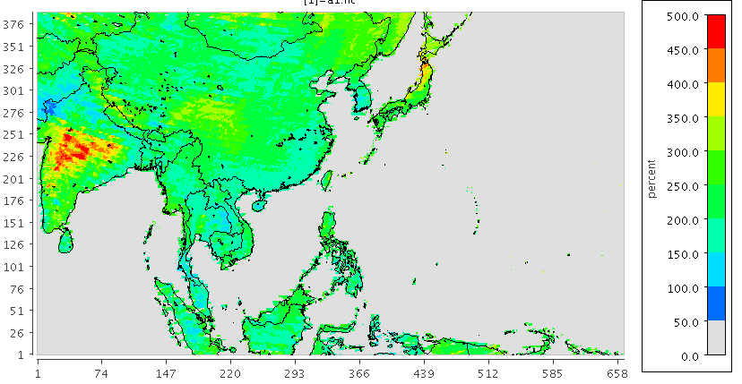圖 d01範圍表土0~5cm之CEC(mmolc/Kg)

Reading 2015 250m resolution Global GeoTiff’s

由前述解析結果顯示，在濱海邊界上並不是對得很整齊，陸地內部數據正確性也堪慮。
另由isric網站找到全球GeoTiff檔，即使經壓縮，每檔仍有2.6G，數據有些多，但圖面看來顯然較佳。
同時納入所有資料，除了pivot_table之外，其餘處理似無法啟動多工模式，整體處理效率會較低。
單一程式即使用到近1/3的記憶體，即使OS層級的多工也受到限制。
使用python的multiprocessing也無法提高效率

Downloading Scripts

for s in CECSOL PHIHOX WWP;do
for d in {1..6};do 
tif=${s}_M_sl${d}_250m_ll.tif
if [ -e $tif ];then continue;fi
pth=https://files.isric.org/soilgrids/former/2017-03-10/data/$tif
wget -q $pth
done
done

tiff2nc

為節省記憶體的使用，在1d階段就進行座標點的篩選，再行擴張np.mesh
數據轉移後將之前的容器清空
此處直接對網格內之值進行平均，不需再記錄筆數。

def tif2nc(tif_name,nc_name,lev):
  from pandas import DataFrame, pivot_table
  import numpy as np
  import netCDF4
  from pyproj import Proj
  import rasterio

  img = rasterio.open(tif_name)
  nx,ny,nz,nodata=img.width,img.height,img.count,img.profile['nodata']
  if nz!=1:return -1
  dx,x0,dy,y0=[img.profile['transform'][i] for i in [0,2,4,5]]
  lon_1d=np.array([x0+dx*i for i in range(nx)])
  lat_1d=np.array([y0+dy*i for i in range(ny)])
  idx0,idx1=np.where((lat_1d>=-10)&(lat_1d<=50))[0],np.where((lon_1d>=60)&(lon_1d<=180))[0]
  data=img.read()[0,:,:]
  img=0 #clean_up the memory
  lonm, latm = np.meshgrid(lon_1d[idx1[:]], lat_1d[idx0[:]])
  i1,i0=np.meshgrid(idx1[:], idx0[:])
  DD={'lon':lonm.flatten(),'lat':latm.flatten(),'val':data[i0.flatten(),i1.flatten()]}
  img,lonm,latm,data=0,0,0,0 #clean_up the memory
  df=DataFrame(DD)
  df=df.loc[df.val != nodata].reset_index(drop=True)
  
  nc = netCDF4.Dataset(nc_name, 'r+')
  pnyc = Proj(proj='lcc', datum='NAD83', lat_1=nc.P_ALP, lat_2=nc.P_BET,lat_0=nc.YCENT, lon_0=nc.XCENT, x_0=0, y_0=0.0)
  V=[list(filter(lambda x:nc.variables[x].ndim==j, [i for i in nc.variables])) for j in [1,2,3,4]]
  nt,nlay,nrow,ncol=(nc.variables[V[3][0]].shape[i] for i in range(4))

  #d00範圍：北緯-10~50、東經60~180。'area': [50, 60, -10, 180,],
  x,y=pnyc(list(df.lon),list(df.lat), inverse=False) #taking time, can not parallelize
  x,y=np.array(x),np.array(y)
  df['ix']=np.array((x-nc.XORIG)/nc.XCELL,dtype=int)
  df['iy']=np.array((y-nc.YORIG)/nc.YCELL,dtype=int)
  x,y=0,0 #clean_up the memory
  df=df.loc[(df.ix>=0)&(df.ix<ncol)&(df.iy>=0)&(df.iy<nrow)].reset_index(drop=True)
  df['ixy']=[str(i)+'_'+str(j) for i,j in zip(df.ix,df.iy)]
  pv=pivot_table(df,index='ixy',values='val',aggfunc=np.mean).reset_index()
  df=0 #clean_up the memory
  pv['ix']=[int(i.split('_')[0]) for i in pv.ixy]
  pv['iy']=[int(i.split('_')[1]) for i in pv.ixy]
  var=np.zeros(shape=(nrow,ncol))
  var[pv.iy,pv.ix]=pv.val
  nc[V[3][0]][0,lev,:,:]=var[:,:]
  nc.close()
  return 0

pH Averaging

pH的定義是水中氫離子濃度的負log₁₀值，因此在平均、內插時不能直接進行，須轉成原本定義，用氫離子濃度進行計算後，再轉成pH值。
轉換過程中因避開無值部分，需先線性化，又因記憶體太大，須多步驟進行：
1. ISRIC提供的數據是0.1pH，因此要先除10
2. 取冪次方只能針對array，df.series太大了直接取次方會有問題。
3. 以氫離子濃度進行pivot_table(取網格內所有值之平均值)
4. array=df.series，可以進行轉換。還是要轉成array才能進行log計算。
5. 再次針對有數值的部分進行線性化，否則0值取-log10會得到NaN。

  a=np.array(df.val)/10.
  df.val=10**(-a)
  pv=pivot_table(df,index='ixy',values='val',aggfunc=np.mean).reset_index()
  a,df=0 #clean_up the memory
  pv['ix']=[int(i.split('_')[0]) for i in pv.ixy]
  pv['iy']=[int(i.split('_')[1]) for i in pv.ixy]
  var=np.zeros(shape=(nrow,ncol))
  var[pv.iy,pv.ix]=pv.val
  idx=np.where(var>0)
  a=-np.log10(var[idx[0][:],idx[1][:]])
  var[idx[0][:],idx[1][:]]=a[:]

Units

NAME	Units	Content	Range
CECSOL	cmolc/kg	Cation exchange capacity of soil	~50
PHIHOX	0.1PH	30~100
WWP	v%	Derived available soil water capacity (volumetric fraction) until wilting point	6~55

Results


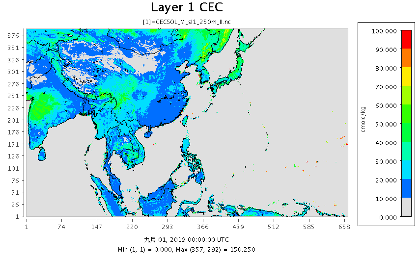圖 d01範圍表土0cm之CEC(cmolc/Kg)

pH averaging scheme

Wilting Point

The physical definition of the wilting point, symbolically expressed as θpwp or θwp, is said by convention as the water content at −1,500 kPa (−15 bar) of suction pressure. wiki
SoilGrids250m 2017-03 - Derived available soil water capacity (volumetric fraction) until wilting point Derived available soil water capacity (volumetric fraction) until wilting point at 7 standard depths predicted using the global compilation of soil ground observations. Accuracy assessement of the maps is availble in Hengl et at. (2017) DOI: 10.1371/journal.pone.0169748. Data provided as GeoTIFFs with internal compression (co=’COMPRESS=DEFLATE’). Measurement units: v%. ISRIC

Field Capacity

Field Capacity is the amount of soil moisture or water content held in the soil after excess water has drained away and the rate of downward movement has decreased. This usually takes place 2–3 days after rain or irrigation in pervious soils of uniform structure and texture. The physical definition of field capacity (expressed symbolically as θfc) is the bulk water content retained in soil at −33 kPa (or −0.33 bar) of hydraulic head or suction pressure. The term originated from Israelsen and West[1] and Frank Veihmeyer and Arthur Hendrickson.[2]
Veihmeyer and Hendrickson[3] realized the limitation in this measurement and commented that it is affected by so many factors that, precisely, it is not a constant (for a particular soil), yet it does serve as a practical measure of soil water-holding capacity. Field capacity improves on the concept of moisture equivalent by Lyman Briggs. Veihmeyer & Hendrickson proposed this concept as an attempt to improve water-use efficiency for farmers in California during 1949.[4]
Field capacity is characterized by measuring water content after wetting a soil profile, covering it (to prevent evaporation) and monitoring the change soil moisture in the profile. Water content when the rate of change is relatively small is indicative of when drainage ceases and is called Field Capacity, it is also termed drained upper limit (DUL).
Lorenzo A. Richards and Weaver[5] found that water content held by soil at a potential of −33 kPa (or −0.33 bar) correlate closely with field capacity (−10 kPa for sandy soils).

Porosity

isric porosity

有關孔隙率isric網站只有提供0.5度解析度之WISE derived soil properties，是個資料庫查詢系統，資料以.dbf形式儲存。
檔案共有10種土壤(SOIL1~10)、10種面積(AREA1~10)、20種總孔隙率TPOR_?T、TPOR_?S(?1~10)、再加SNUM共41欄。
- SNUM為1~45948的整數，為WISE系統內部專用碼(空間對照)
- AREA為對應該土壤的面積比例(%)
- TPOR_T：top soil(0~30cm)/TPOR_S:sub soil(30~100cm)
結論：ArcGIS檔案(.lyr、.adf)無法由外部破解，無法讀取SNUM的對照位置

NASA GLDAS

說明、檔案位置
因解析度只有0.25度，小於15Km，因此必須用內插方式(scipy.interpolate.griddata)轉換座標。

from pandas import DataFrame, pivot_table
import numpy as np
import netCDF4
from pyproj import Proj
from scipy.interpolate import griddata

fname='GLDASp5_porosity_025d.nc4'
nc = netCDF4.Dataset(fname, 'r')
v='GLDAS_porosity'
data=nc[v][0,:,:]
data=np.where(data>0,data,0)
lon_1d=nc['lon'][:]
lat_1d=nc['lat'][:]
lonm, latm = np.meshgrid(lon_1d, lat_1d)
x,y=pnyc(lonm,latm, inverse=False)

fname='GLDASp5_porosityCWBWRF_15Km.nc'
nc = netCDF4.Dataset(fname, 'r+')
pnyc = Proj(proj='lcc', datum='NAD83', lat_1=nc.P_ALP, lat_2=nc.P_BET,lat_0=nc.YCENT, lon_0=nc.XCENT, x_0=0, y_0=0.0)
V=[list(filter(lambda x:nc.variables[x].ndim==j, [i for i in nc.variables])) for j in [1,2,3,4]]
nt,nlay,nrow,ncol=(nc.variables[V[3][0]].shape[i] for i in range(4))
x1d=[nc.XORIG+nc.XCELL*i for i in range(ncol)]
y1d=[nc.YORIG+nc.YCELL*i for i in range(nrow)]
x1,y1=np.meshgrid(x1d,y1d)
maxx,maxy=x1[-1,-1],y1[-1,-1]
minx,miny=x1[0,0],y1[0,0]
boo=(abs(x) <= (maxx - minx) /2+nc.XCELL*10) & (abs(y) <= (maxy - miny) /2+nc.YCELL*10)
idx = np.where(boo)
mp=len(idx[0])
xyc= [(x[idx[0][i],idx[1][i]],y[idx[0][i],idx[1][i]]) for i in range(mp)]

var=np.zeros(shape=(nrow,ncol))
c = data[idx[0][:],idx[1][:]]
var[:,: ] = griddata(xyc, c[:], (x1, y1), method='linear')
nc[V[3][0]][0,lev,:,:]=var[:,:]
nc.close()

Results


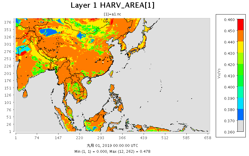圖 d01範圍表土0cm之Porosity(Vv/Vs_Fraction)

Reference

W. J. Rawls, D. L. Brakensiek, K. E. Saxtonn (1982). Estimation of Soil Water Properties. Transactions of the ASAE. 25, 1316–1320. https://doi.org/10.13031/2013.33720
- lookup table
Aliku, O., Oshunsanya, S.O. (2016). Establishing relationship between measured and predicted soil water characteristics using SOILWAT model in three agro-ecological zones of Nigeria. Geosci. Model Dev. Discuss. https://doi.org/10.5194/gmd-2016-165
- Field Capacity moisture (33 kPa), %v